[Δ]ij= 
The Laplacian matrix, denoted by L, is a real symmetric V × V matrix that may also be considered as a kind of augmented vertex-adjacency matrix. It is defined as the following difference matrix [159]:
L = Δ - vA (27)
where Δ is a diagonal matrix of dimension V × V whose diagonal entries are the vertex-degrees:
[Δ]ij= |
d(i) if i = j |
| 0 otherwise (28) |
where d(i) is the degree of the vertex i. This matrix is also called the vertex-degree matrix [21].
The entries of the Laplacian matrix are as follows:
[L]ij= |
-1 if vertices i and j are adjacent |
| d(i) if i = j | |
| 0 otherwise (29) |
It should be noted that the smallest eigenvalue of L is always equal to zero, as a consequence of the special structure of the Laplacian matrix.
The Laplacian matrix is sometimes also called Kirchhoff matrix [159-162], due to its role in the matrix-tree theorem [19], implicit [163] in electrical-network work of Kirchhoff [164; in his paper Kirchhoff also introduced the concept of the spanning tree though he did not use this term]. It is also known as the admittance matrix [19]. However, the name Laplacian matrix appears to be more appropriate since this matrix is just the matrix of a discrete Laplacian operator, which is one of the basic differential operators in quantum chemistry and beyond. Below we give the Laplacian matrix of the vertex-labeled graph G1 (see structure A in Figure 2).
L(G1)= |
1 |
-1 |
0 |
0 |
0 |
0 |
0 |
||
-1 |
2 |
-1 |
0 |
0 |
0 |
0 |
|||
0 |
-1 |
3 |
-1 |
0 |
-1 |
0 |
|||
0 |
0 |
-1 |
2 |
-1 |
0 |
0 |
|||
0 |
0 |
0 |
-1 |
2 |
-1 |
0 |
|||
0 |
0 |
-1 |
0 |
-1 |
3 |
-1 |
|||
0 |
0 |
0 |
0 |
0 |
-1 |
1 |
The Laplacian matrix is used to enumerate the number of spanning trees [165] Let us remind the reader that a spanning tree of a graph G is a connected acyclic subgraph containing all the vertices of G [12].
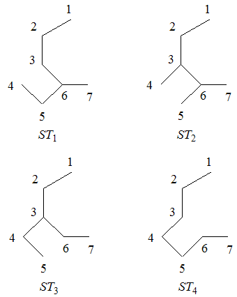
If a graph contains a single cycle, then the number of spanning trees is simply equal to the size of the cycle. Thus, since the graph G1 contains a 4-membered cycle (see Figure 1), it possesses 4 spanning trees, denoted by STn (n=1,2,3,4). They are depicted in Figure 20. These will be utilized later on in section 4.15.
Figure 20. Labeled spanning trees of G1.
When a polycyclic graph G is considered, then obtaining the number of spanning trees is complicated. One needs first to compute the Laplacian spectrum and then to use it in the following counting formula, based on the matrix-tree theorem, in order to get the number of spanning trees of G [159]:
t(G)=(1/V) |
V | λi |
(30) |
| Π | |||
| i=2 |
where t(G) is the number of spanning trees of G and λi (i=2,...V) is the eigenvalue of the Laplacian matrix. There is a reason why the multiplication of eigenvalues in this formula starts with λ2 - the smallest member of the Laplacian spectrum λ1 is always zero.
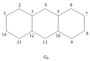
We will exemplify the use of formula (30) to enumerate the spanning trees of a graph representing the carbon skeleton of anthracene. This graph is shown in Figure 21.
Figure 21. Labeled anthracene graph.
The Laplacian spectrum of the anthracene graph is: {0.0000, 0.1981, 0.7530, 0.8402, 1.1206, 1.5500, 1.6207, 2.4450, 3.2470, 3.3473, 3.4919, 3.8019, 4.5321, 5.0472}. Now, we enter these numbers in formula (30) to get the number of spanning trees of the anthracene graph: 204. Spanning trees have found use in ring current calculations on conjugated systems [41] and in assessing the complexity of molecules and graphs, and reaction mechanisms [e.g., 57,165,166]. In the next section we will show a simpler approach to the enumeration of the number of spanning trees of polycyclic graphs.
Several topological indices based on the Laplacian matrix have been proposed, besides the number of spanning trees [159,167], the Mohar indices [159,168], the Wiener index of trees [159,168-170] , the quasi-Wiener index [171] and spanning-tree density and reciprocal spanning-tree density [172] .